# import modulesimportnumpyasnpimportmatplotlib.pyplotasplt# functionsdeftest_plot(full_data,missing_data,title,save_path):"""
Plot the first 3 dimensions of the first sample, comparing full data and missing data.
"""fig,axes=plt.subplots(3,1,figsize=(12,8),sharex=True)forjinrange(3):axes[j].plot(full_data[0,j],color='gray',label='full data',alpha=0.6)axes[j].plot(missing_data[0,j],color='red',label=title)axes[j].set_ylabel(f'Dim {j}')axes[j].legend()plt.suptitle(title)plt.xlabel('Time')plt.tight_layout()plt.savefig(f"{save_path}.png",dpi=300)plt.show()
# Training configurationbatch_size:50# Batch sizeoutput_directory:"./results/checkpoint"# Output directory for checkpoints and logsckpt_iter:"max"# Checkpoint mode (max or min)iters_per_ckpt:100# Checkpoint frequency (number of epochs)iters_per_logging:100# Log frequency (number of iterations)n_iters:10000# Maximum number of iterationslearning_rate:0.002# Learning rate# Additional training settingsonly_generate_missing:true# Generate missing values onlyuse_model:2# Model to use for trainingmasking:"forecast"# Masking strategy for missing valuesmissing_k:5# Number of missing values# Data pathsdata:train_path:"./datasets/real_time_by_autoFRK/pollutants_train.npy"# Path to training data
wavenet:# WaveNet model parametersinput_channels:26# Number of input channelsoutput_channels:26# Number of output channelsresidual_layers:32# Number of residual layersresidual_channels:128# Number of channels in residual blocksskip_channels:128# Number of channels in skip connections# Diffusion step embedding dimensionsdiffusion_step_embed_dim_input:64# Input dimensiondiffusion_step_embed_dim_hidden:512# Middle dimensiondiffusion_step_embed_dim_output:512# Output dimension# Structured State Spaces sequence model (S4) configurationss4_max_sequence_length:2000# Maximum sequence lengths4_state_dim:64# State dimensions4_dropout:0.0# Dropout rates4_bidirectional:true# Whether to use bidirectional layerss4_use_layer_norm:true# Whether to use layer normalizationdiffusion:# Diffusion model parametersT:200# Number of diffusion stepsbeta_0:0.0001# Initial beta valuebeta_T:0.02# Final beta value
用於填補的設定檔。
1
2
3
4
5
6
7
8
9
10
11
12
13
14
15
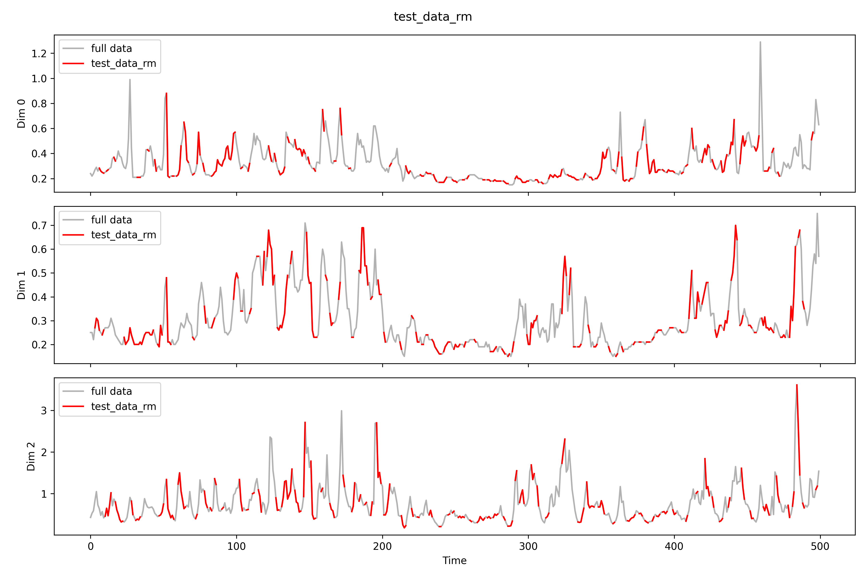
# Inference configurationbatch_size:50# Batch size for inferenceoutput_directory:"./results/checkpoint/rm"# Output directory for inference resultsckpt_path:"./results/checkpoint"# Path to checkpoint for inferencetrials:1# Replications# Additional training settingsonly_generate_missing:true# Generate missing values onlyuse_model:2# Model to use for trainingmasking:"forecast"# Masking strategy for missing valuesmissing_k:200# Number of missing values# Data pathsdata:test_path:"./datasets/real_time_by_autoFRK/pollutants_test_rm.npy"# Path to test data
defget_mask_forecast(sample:torch.Tensor,k:int)->torch.Tensor:"""
Get mask of same segments (black-out missing) across channels based on k.
Args:
sample (torch.Tensor): Tensor of shape [# of samples, # of channels].
k (int): Number of missing values.
Returns:
torch.Tensor: Mask of sample's shape where 0's indicate missing values to be imputed, and 1's indicate preserved values.
"""#mask = torch.ones_like(sample) # Initialize mask with all ones# Calculate the indices of missing values#s_nan = torch.arange(mask.shape[0] - k, mask.shape[0])# Apply mask for each channel#for channel in range(mask.shape[1]):# mask[s_nan, channel] = 0mask=(~torch.isnan(sample)).float()# replace only missing valuesreturnmask
defget_mask_forecast(sample:torch.Tensor,k:int)->torch.Tensor:"""
Get mask of same segments (black-out missing) across channels based on k.
Args:
sample (torch.Tensor): Tensor of shape [# of samples, # of channels].
k (int): Number of missing values.
Returns:
torch.Tensor: Mask of sample's shape where 0's indicate missing values to be imputed, and 1's indicate preserved values.
"""#mask = torch.ones_like(sample) # Initialize mask with all ones# Calculate the indices of missing values#s_nan = torch.arange(mask.shape[0] - k, mask.shape[0])# Apply mask for each channel#for channel in range(mask.shape[1]):# mask[s_nan, channel] = 0mask=(~torch.isnan(sample)).float()returnmask
這裡也需要修改,讓缺值部分填入 0 ,使得程式碼能進行填補( NA 無法進行數值運算,會報錯)。此段程式碼位於 /SSSD_CP-main/sssd/inference/generator.py 。
新增了 batch = torch.nan_to_num(batch, nan=0.0) # Replace NaN with 0.0 。
defgenerate(self)->list:"""Generate samples using the given neural network model."""all_mses=[]all_mapes=[]forindex,(batch,)inenumerate(self.dataloader):batch=batch.to(self.device)mask=self._update_mask(batch)iftorch.isnan(mask).any():# debugprint(f"[Batch {index}] NaN in mask!")batch=torch.nan_to_num(batch,nan=0.0)# Replace NaN with 0.0iftorch.isnan(batch).any():# debugprint(f"[NaN DETECTED] Batch {index} has NaNs!")batch=batch.permute(0,2,1)generated_series=(sampling(net=self.net,size=batch.shape,diffusion_hyperparams=self.diffusion_hyperparams,cond=batch,mask=mask,only_generate_missing=self.only_generate_missing,device=self.device,).detach().cpu().numpy())ifnp.isnan(generated_series).any():# debugprint("[NaN DETECTED] in generated_series")print("Locations:",np.argwhere(np.isnan(generated_series)))batch=batch.detach().cpu().numpy()mask=mask.detach().cpu().numpy()mse=mean_squared_error(batch[~mask.astype(bool)],generated_series[~mask.astype(bool)])mape=mean_absolute_percentage_error(batch[~mask.astype(bool)],generated_series[~mask.astype(bool)])all_mses.append(mse)all_mapes.append(mape)results={"imputation":generated_series,"original":batch,"mask":mask,}self._save_data(results,index)returnall_mses,all_mapes
# test imputationimportosimportnumpyasnpimportmatplotlib.pyplotaspltfromtqdmimporttqdmtest_data=np.load(r'real_time\pollutants_test.npy').transpose(0,2,1)## functionsdefimputation_plot(full_data,missing_data,imputation_data,title,save_path):"""
Plot the first 3 dimensions of the first sample, comparing full data and missing data.
"""show_dims=2fig,axes=plt.subplots(show_dims,1,figsize=(12,8),sharex=True)#imputation_data = np.where(np.isnan(missing_data), imputation_data, np.nan)forjinrange(show_dims):axes[j].plot(full_data[0,j],color='gray',label='full data',alpha=0.6)axes[j].plot(imputation_data[0,j],color='orange',label='imputation data',alpha=0.6)axes[j].plot(missing_data[0,j],color='red',label=title)axes[j].set_ylabel(f'Dim {j}')axes[j].legend()plt.suptitle(title)plt.xlabel('Time')plt.tight_layout()plt.savefig(f"{save_path}.png",dpi=300)#plt.show()defimputation_plot_each_dim(full_data,missing_data,imputation_data,title,save_dir):"""
Plot each dimension of the first sample separately, comparing full data, missing data, and imputation data.
Save each plot as a separate file.
"""num_dims=full_data.shape[1]os.makedirs(save_dir,exist_ok=True)# 確保保存目錄存在forjintqdm(range(num_dims)):fig,ax=plt.subplots(figsize=(12,4))ax.plot(full_data[0,j],color='gray',label='full data',alpha=0.6)ax.plot(imputation_data[0,j],color='orange',label='imputation data',alpha=0.6)ax.plot(missing_data[0,j],color='red',label=title)ax.set_ylabel(f'Dim {j}')ax.set_xlabel('Time')ax.set_title(f'{title} - Dimension {j}')# 圖例放到圖外ax.legend(loc='center left',# 圖例在圖的左側中央(搭配下面這行)bbox_to_anchor=(1,0.5)# (x, y):x=1是圖的最右邊,往右推一點)fig.tight_layout(rect=[0,0,0.85,1])# 調整畫布大小,右邊留空給圖例save_path=os.path.join(save_dir,f"{title}_dim{j}.png")plt.savefig(save_path,dpi=300)plt.close(fig)# 不然畫一堆圖會記憶體爆掉
rm
 1
 2
 3
 4
 5
 6
 7
 8
 9
10
11
12
13
14
15
16
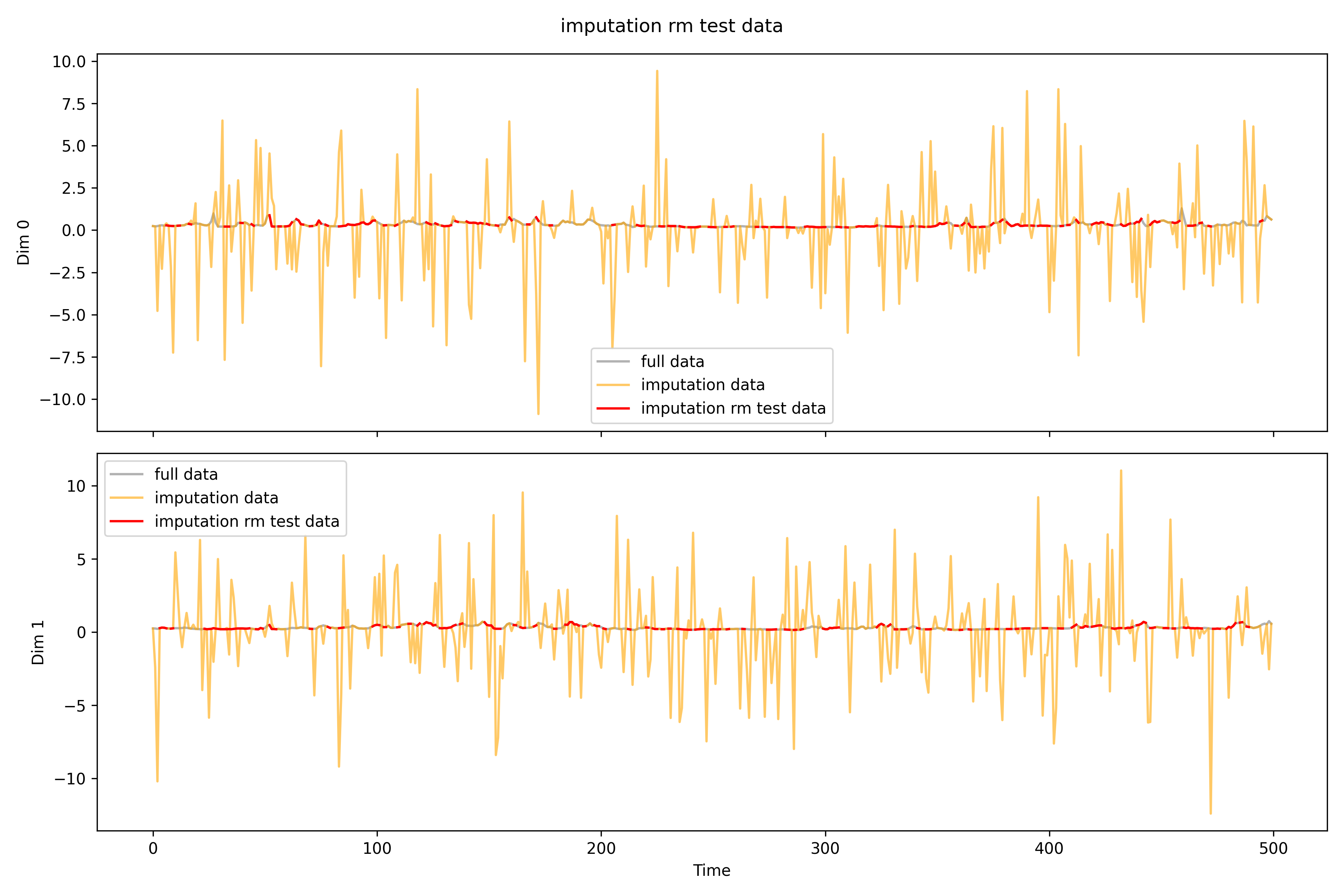
## rmfilename=r'real_time\imputation\imputation0_rm.npy'rm_data=np.load(filename)print(f'Shape: {rm_data.shape}')print(f'NAs: {np.isnan(rm_data).sum()}')# print(rm_data[0, 0])print(f'MSPE for all: {((test_data-rm_data)**2).mean()}')test_data_rm=np.load(r'real_time\pollutants_test_rm.npy').transpose(0,2,1)print(f'MSPE only for missing: {((test_data[np.isnan(test_data_rm)]-rm_data[np.isnan(test_data_rm)])**2).mean()}')imputation_plot(test_data,test_data_rm,rm_data,'imputation rm test data',r'real_time\imputation\imputation0_rm')imputation_plot_each_dim(test_data,test_data_rm,rm_data,'imputation rm test data',r'real_time\imputation\imputation0_rm\each_dim')# test_data[0, 0][1:10]# test_data_rm[0, 0][1:10]# rm_data[0, 0][1:10]
執行結果參考
1
2
3
4
5
Shape: (5, 26, 500)NAs: 0MSPE for all: 5.630354000694568
MSPE only for missing: 7.2555356208301784
100%|████████████████████████████████████████████████████████████████████████████████████████████████████████████████████| 26/26 [00:13<00:00, 1.95it/s]
imputation rm 。
所有測站填補情形如下。
gallery_made_with_nanogallery2-1-rm
rbm
 1
 2
 3
 4
 5
 6
 7
 8
 9
10
11
12
13
14
15
16
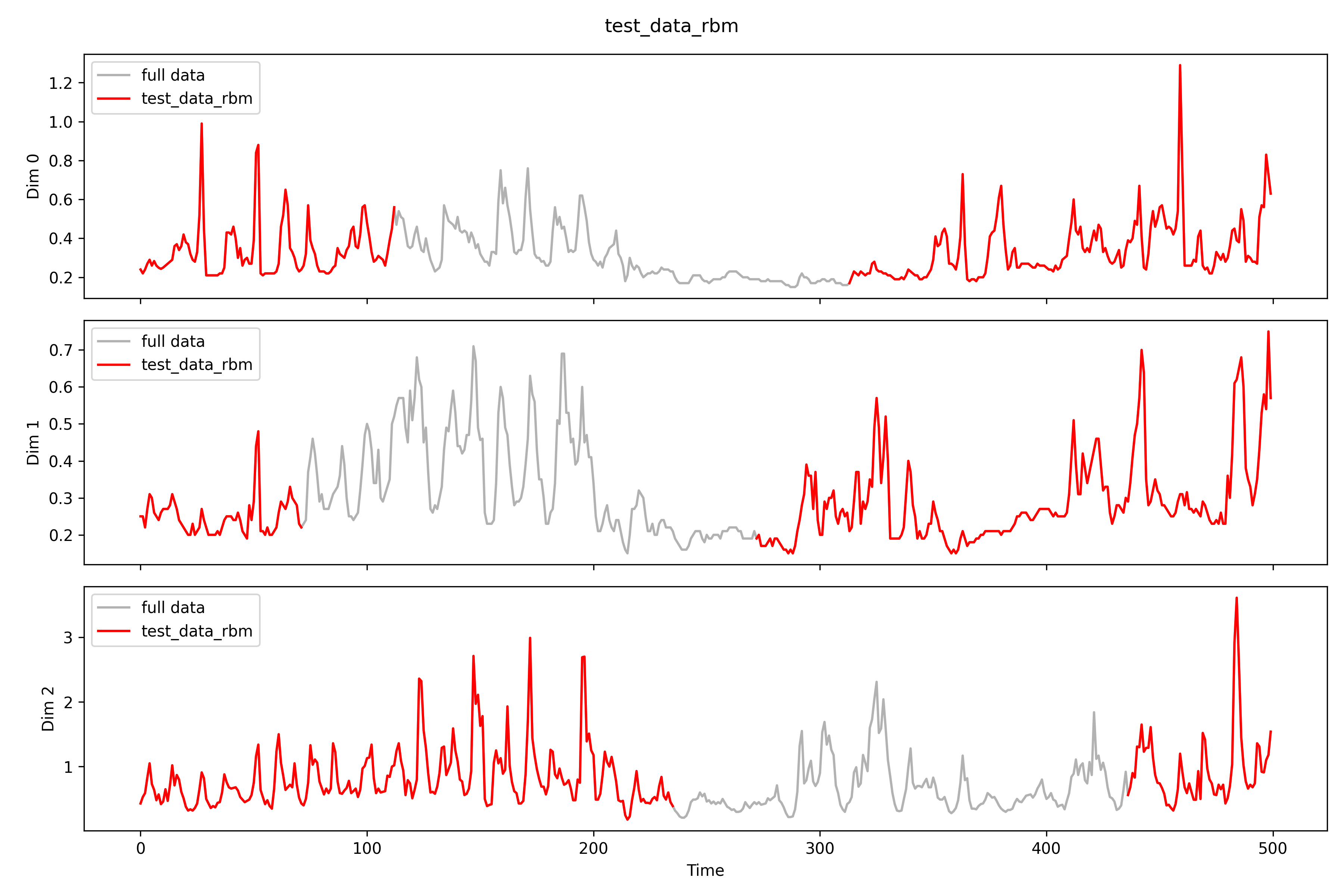
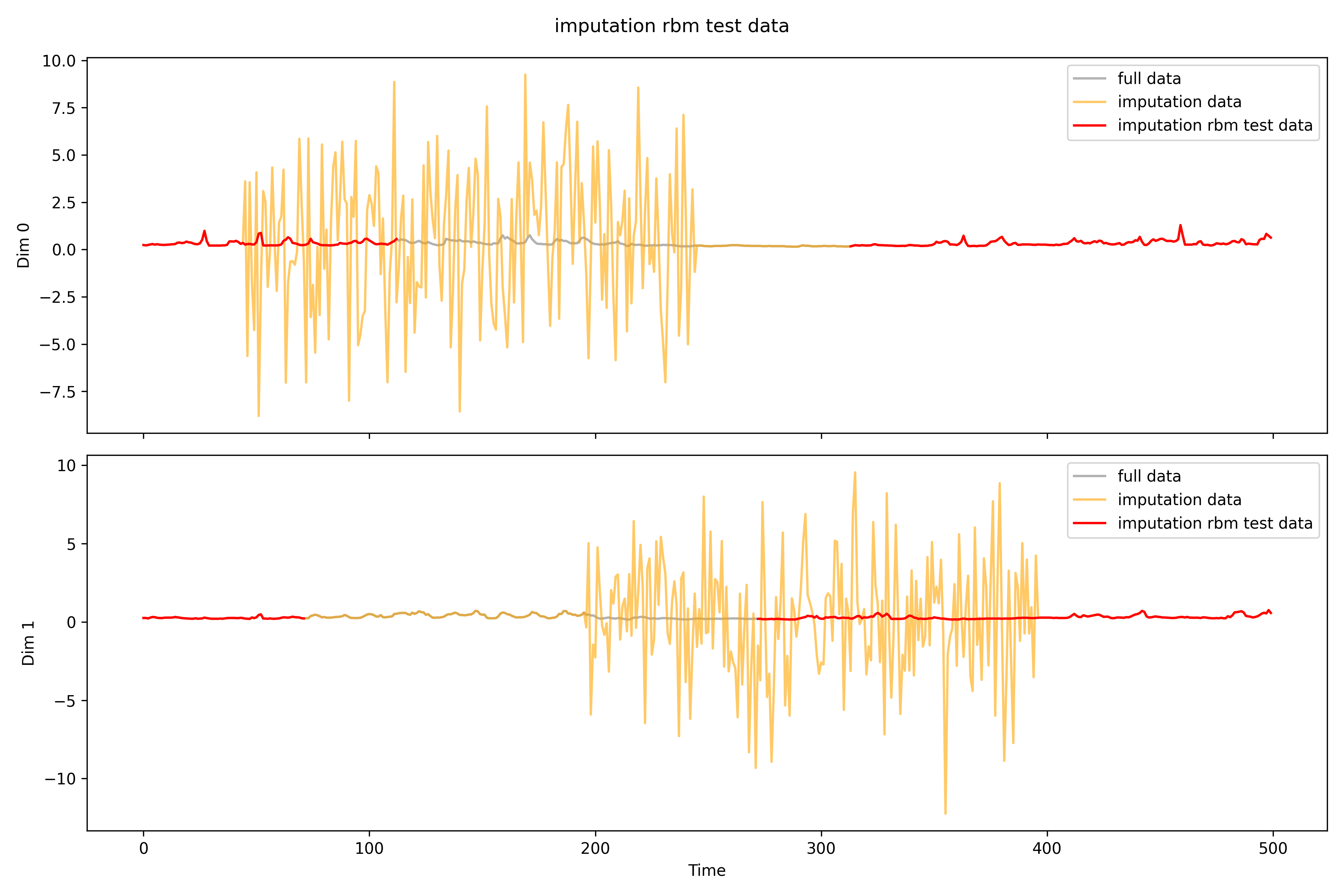
## rbmfilename=r'real_time\imputation\imputation0_rbm.npy'rbm_data=np.load(filename)print(f'Shape: {rbm_data.shape}')print(f'NAs: {np.isnan(rbm_data).sum()}')# print(rbm_data[0, 0])print(f'MSPE for all: {((test_data-rbm_data)**2).mean()}')test_data_rbm=np.load(r'real_time\pollutants_test_rbm.npy').transpose(0,2,1)print(f'MSPE only for missing: {((test_data[np.isnan(test_data_rbm)]-rbm_data[np.isnan(test_data_rbm)])**2).mean()}')imputation_plot(test_data,test_data_rbm,rbm_data,'imputation rbm test data',r'real_time\imputation\imputation0_rbm')imputation_plot_each_dim(test_data,test_data_rbm,rbm_data,'imputation rbm test data',r'real_time\imputation\imputation0_rbm\each_dim')# test_data[0, 0][1:10]# test_data_rbm[0, 0][1:10]# rbm_data[0, 0][1:10]
執行結果參考
1
2
3
4
5
Shape: (5, 26, 500)NAs: 0MSPE for all: 5.67021524531403
MSPE only for missing: 8.879126539941137
100%|████████████████████████████████████████████████████████████████████████████████████████████████████████████████████| 26/26 [00:13<00:00, 1.97it/s]
imputation rbm 。
所有測站填補情形如下。
gallery_made_with_nanogallery2-2-rbm
bm
1
2
3
4
5
6
7
8
9
10
11
12
13
14
15
16
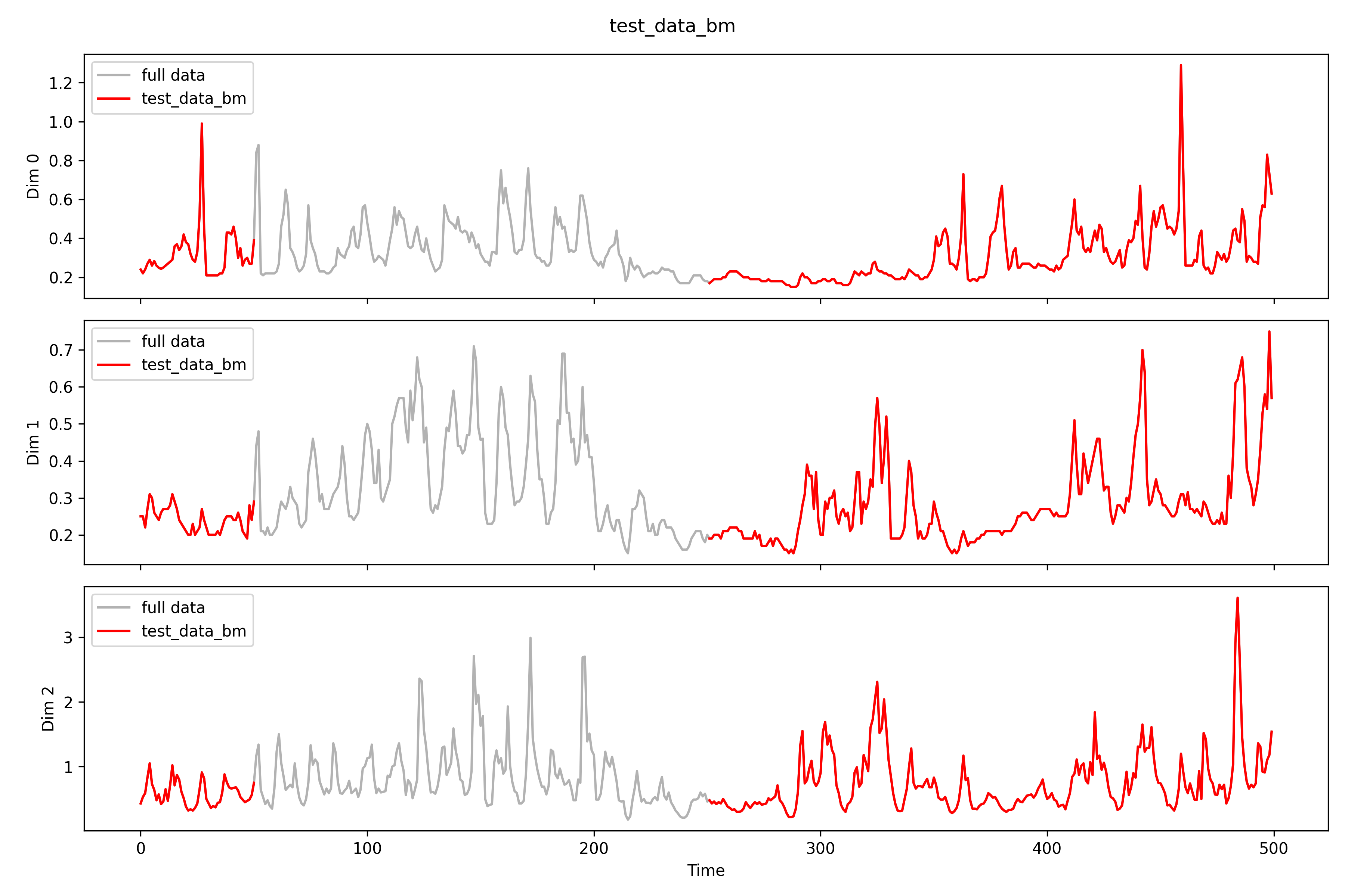
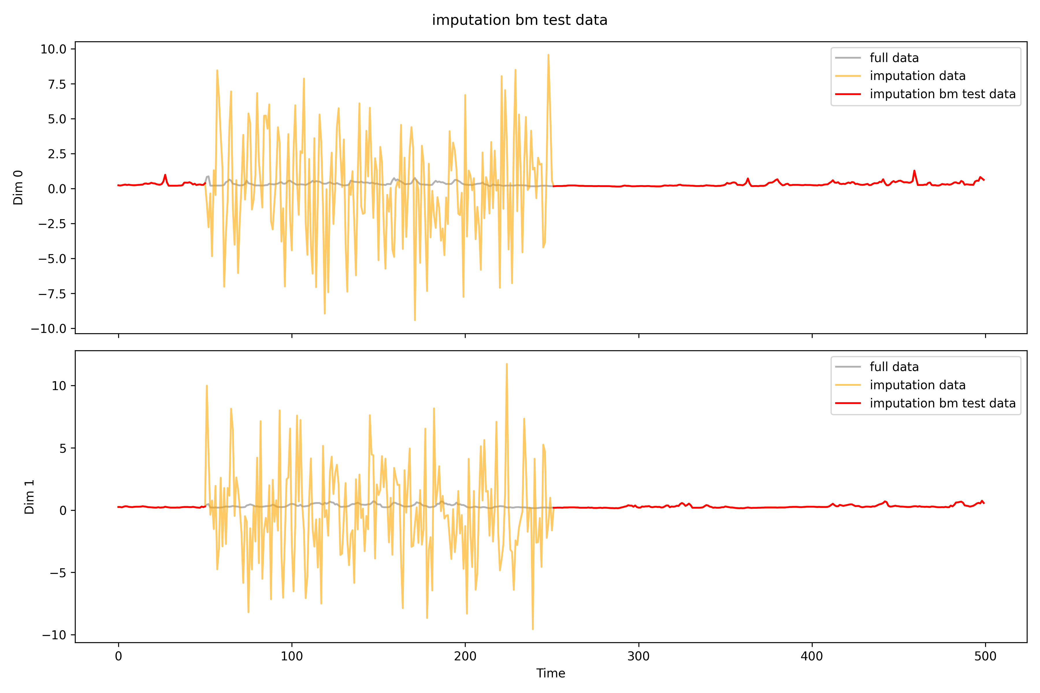
## bmfilename=r'real_time\imputation\imputation0_bm.npy'bm_data=np.load(filename)print(f'Shape: {bm_data.shape}')print(f'NAs: {np.isnan(bm_data).sum()}')# print(bm_data[0, 0])print(f'MSPE for all: {((test_data-bm_data)**2).mean()}')test_data_bm=np.load(r'real_time\pollutants_test_bm.npy').transpose(0,2,1)print(f'MSPE only for missing: {((test_data[np.isnan(test_data_bm)]-bm_data[np.isnan(test_data_bm)])**2).mean()}')imputation_plot(test_data,test_data_bm,bm_data,'imputation bm test data',r'real_time\imputation\imputation0_bm')imputation_plot_each_dim(test_data,test_data_bm,bm_data,'imputation bm test data',r'real_time\imputation\imputation0_bm\each_dim')# test_data[0, 0][1:10]# test_data_bm[0, 0][1:10]# bm_data[0, 0][1:10]
執行結果參考
1
2
3
4
5
Shape: (5, 26, 500)NAs: 0MSPE for all: 5.733927828240412
MSPE only for missing: 14.33481884698311
100%|████████████████████████████████████████████████████████████████████████████████████████████████████████████████████| 26/26 [00:13<00:00, 1.95it/s]
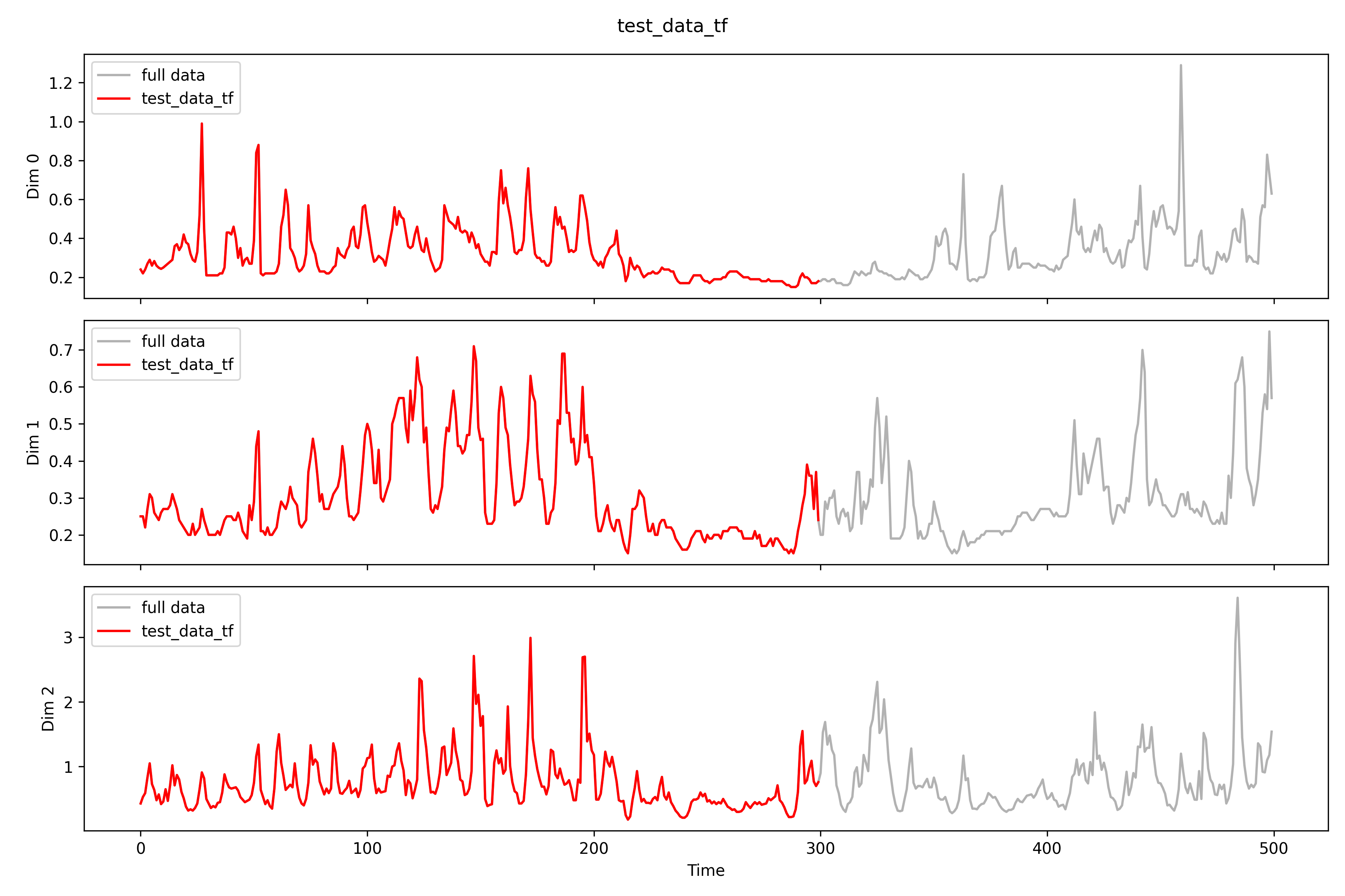
imputation bm 。
所有測站填補情形如下。
gallery_made_with_nanogallery2-3-bm
tf
 1
 2
 3
 4
 5
 6
 7
 8
 9
10
11
12
13
14
15
16
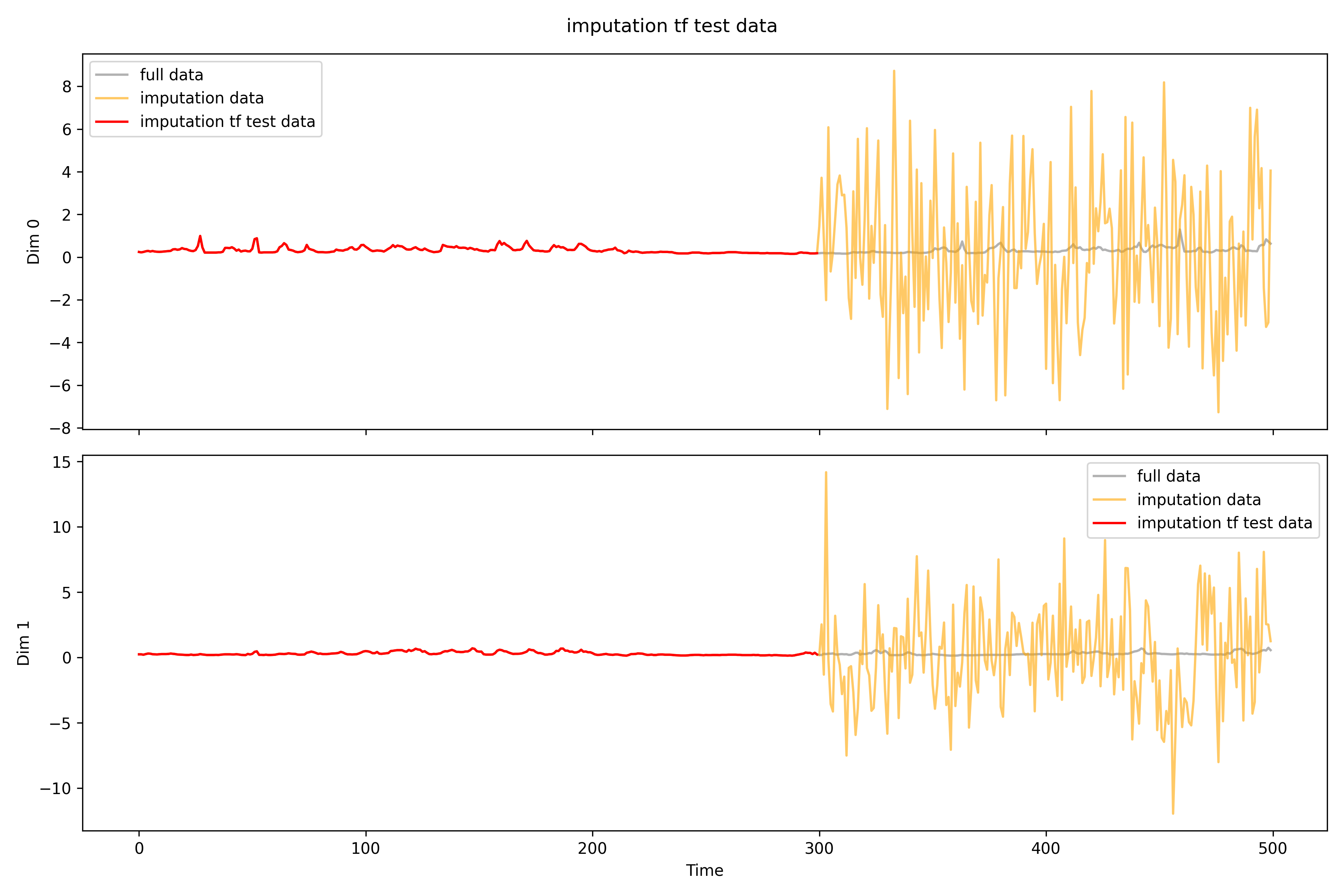
## tffilename=r'real_time\imputation\imputation0_tf.npy'tf_data=np.load(filename)print(f'Shape: {tf_data.shape}')print(f'NAs: {np.isnan(tf_data).sum()}')# print(tf_data[0, 0])print(f'MSPE for all: {((test_data-tf_data)**2).mean()}')test_data_tf=np.load(r'real_time\pollutants_test_tf.npy').transpose(0,2,1)print(f'MSPE only for missing: {((test_data[np.isnan(test_data_tf)]-tf_data[np.isnan(test_data_tf)])**2).mean()}')imputation_plot(test_data,test_data_tf,tf_data,'imputation tf test data',r'real_time\imputation\imputation0_tf')imputation_plot_each_dim(test_data,test_data_tf,tf_data,'imputation tf test data',r'real_time\imputation\imputation0_tf\each_dim')# test_data[0, 0][1:10]# test_data_tf[0, 0][1:10]# tf_data[0, 0][1:10]
執行結果參考
1
2
3
4
5
Shape: (5, 26, 500)NAs: 0MSPE for all: 5.728256563966483
MSPE only for missing: 14.320640763169513
100%|████████████████████████████████████████████████████████████████████████████████████████████████████████████████████| 26/26 [00:13<00:00, 1.94it/s]